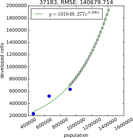
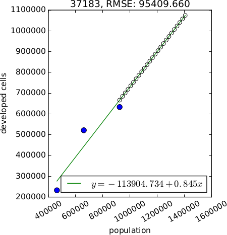
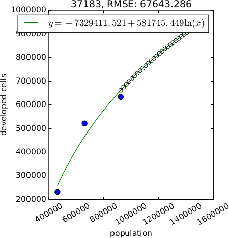
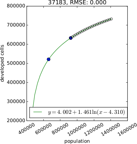
Figure: Example of different relations between population and developed area (generated with option plot). Starting from the left: exponential, linear, logarithmic with 2 unknown variables, logarithmic with 3 unknown variables, exponential approach
The input accepts multiple (at least 2) rasters of developed (category 1) and undeveloped areas (category 0) from different years, ordered by time. For these years, user has to provide the population numbers for each subregion in parameter observed_population as a CSV file. The format is as follows. First column is time (matching the time of rasters used in parameter development) and first row is the category of the subregion. The separator can be set with parameter separator.
year	1	2	...
1985	19860	10980	...
1995	20760	12660	...
2005	21070	13090	...
2015	22000	13940	...
The same table is needed for projected population (parameter projected_population). The categories of the input raster subregions must match the identifiers of subregions in files given in observed_population and projected_population. Parameter simulation_times is a comma separated list of times for which the demand will be computed. The first time should be the time of the developed/undeveloped raster used in r.futures.pga as a starting point for simulation. There is an easy way to create such list using Python:
','.join([str(i) for i in range(2015, 2031)])or Bash:
seq -s, 2015 2030
The format of the output demand table is:
    year	37037	37063	37069	...
    2012	1362	6677	513	...
    2013	1856	4850	1589	...
    2014	1791	5972	903	...
    2015	1743	5497	1094	...
    2016	1722	5388	1022	...
    2017	1690	5285	1077	...
    2018	1667	5183	1029	...
...
where each value represents the number of new developed cells in each step.
It's a standard CSV file with tabulators as separators, so it can be opened
in a text editor or a spreadsheet application if needed.
In case the demand values would be negative (in case of population decrease
or if the relation is inversely proportional) the values are turned into zeros,
since FUTURES does not simulate change from developed to undeveloped sites.
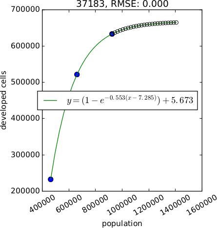
The method parameter allows to choose the type of relation between population and developed area. The available methods include linear, logarithmic (2 options), exponential and exponential approach relation. If more than one method is checked, the best relation is selected based on RMSE. Recommended methods are logarithmic, logarithmic2, linear and exp_approach. Methods exponential approach and logarithmic2 require scipy and at least 3 data points (raster maps of developed area).
An optional output plot is a plot of the relations for each subregion. It allows to more effectively assess the relation suitable for each subregion. Format of the file is determined from the extension and can be for example PNG, PDF, SVG.
Figure: Example of different relations between population and developed area (generated with option plot). Starting from the left: exponential, linear, logarithmic with 2 unknown variables, logarithmic with 3 unknown variables, exponential approach
r.futures.demand development=urban_1992,urban_2001,urban_2011 subregions=counties \
observed_population=population_trend.csv projected_population=population_projection.csv \
simulation_times=`seq -s, 2011 2035` plot=plot_demand.pdf demand=demand.csv
Last changed: $Date$