NAME

DESCRIPTION

This module and its manual page have been written with archaeological predictive modelling (APM) in mind, but should be useful for other cases where presence or absence of objects of interest is to be predicted. In the following text, replace the term "site" with any other name of an object of interest.

A very simple way to calculate a predictive model is using the dst.predict wrapper program.

Introduction

In APM, the FOD is taken to consist of two singleton hypotheses and the set of these two:

H1={"SITE"}

This proposes that an archaeological site is present.

H2={"NO SITE}"

This proposes that no archaeological site is present.

H3={"SITE","NO SITE}"

This proposes that no decision can be made about site presence or absence (uncertainty).

The purpose of r.dst.bpn is to calculate a BPN for these three hypotheses by using only two source of evidences readily available in a GIS-based analysis: (a) a CELL format GRASS raster map that shows categories which are deemed to influence the probability of a site having been established in a location, such as soil type and quality, distance to water, slope etc. and (b) a GRASS vector map which contains the locations of already discovered sites as vector points. The latter are used to sample the raster map in a systematic way. The basic idea is to check for differences in proportions between the sample (cells with sites) and the population (all other cells in the region). These differences are used to quantify the strength of belief (BPN) in each of the FOD's three hypotheses. The output of this program consists of three raster maps, with basename given by the user (option output=) and suffixes ".SITE", ".NOSITE" and ".SITE.NOSITE", which encode the BPNs for the respective hypotheses. These maps can be combined with BPN maps generated from other sources of evidence by dst.combine to calculate the overall belief in H1 or H2 as supported by the given evidence (as well as many other useful metrics derrived from this).

Details of BPN quantification

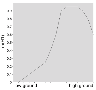
Let us look at an archaeological example: we want to model belief in the presence or absence of a certain type of hillfort settlements at different altitudes (evidence "height") in a topographically varied region of interest. At first glance, the situation looks straight-forward: the higher the terrain, the higher we believe the chance to find that kind of settlement (i.e. m(H1) closer to "1"), as higher locations are better to defend. However, even in this simple case, an adequate BPN function would be more complex. Let us look at a plot of m(H1) vs. "height", as derrived from some archaeologist's subjective belief:

1. Starting at the lowest height, there would first be a flat section that represents the height range of the low lands in which no forts were built.
2. This would be succeeded by a section with gradually steeper inclination as the height approaches a range which the prehistoric builders found optimal.
3. Within this optimal range, the curve flattens out on a high level.
4. Above a certain height however, logistic problems become too great and we do not believe that prehistoric people were able to cope with them beyond a certain point, thus m(H1) falls off towards "0" quickly.

1. a vector points map S with the locations of known sites;
2. a raster map M that represents the evidence (e.g. height).

Likewise, one or more vector point attributes can be chosen to represent "SITE" bias, such as unfounded trust in the location of a site.

The raster evidence map must be fully categorised, i.e. each cell must represent a category (e.g. 1='0 to 5 m', 2='5 to 10 m',...) or be NULL (no data). You can use the r.categorize program to quickly create such a map from any GRASS raster map.

For each category C in the input evidence map M, r.dst.bpn compares the overall cell percentage of C in M (Perc(M)) with the percentage of category C cells that contain a site from S (Perc(S)).
The assumption is that if Perc(M) > Perc(S) at a significant level then the evidence in M and S supports the hypothesis "NO SITE" for all cells in M and if Perc(M) < Perc(S) it supports "SITE". If the difference is found to be of very high signficance, the belief mass assigned to on of these two hypothesis tends towards "1", if it is low, it tends towards "0".

Just how signficant the difference in percentages is depends on (a) the magnitude of the difference (b) the size of the sample and (c) the number of cells in the entire region. This is catered for by calculating a z-statistic for each case. The z-statistic gives the probability of observing a difference in proportions as extreme as Perc(M)-Perc(S) under the assumption that there is no significant difference between Perc(M) and Perc(S). In effect, this gives the probability of making an error when declaring it significant (see "Uncertainty handling" for details on how this affects BPN values). If the total number n of sites in S is greater than 30, this will be derrived from a standard normal distribution, otherwise from a t-distribution with n degrees of freedom.

In addition, if the probability of error exceeds a certain threshold (by default 0.05 or 5%), the belief mass to be shifted will be exponentially weighted, so that more belief mass is shifted increasingly rapidly to the uncertainty hypothesis as the probability of error drops further below the threshold. You can adjust the threshold by using the perror parameter.

Often, one will not be restricted as to what category ranges to choose (e.g. 1, 5 or 10 m intervals for evidence "height"?). If there are too many categories in M, r.dst.bpn will produce an overfitting function and a model based on such BPNs will not be able to generalise well, i.e. its predictions are very likely to be wrong when checked against new data. On the other hand, if there are extremely few categories, the program might not be able to find significant evidence that supports either hypothesis. As a safeguard, a chi-square test is run over all categories. This calculates the probability of making an error when declaring the overall set of percentage differences significant (see "Uncertainty handling" for details on how this affects BPN values).

Another option is to use categories with individual ranges. One could use a priori knowledge about the region's natural zones to create a more significant categorisation manually (using r.support):

	Cat.	Range		Label
	1	0-1000		plains and valleys
	2	1000-1500	hills
	3	1500-1700	mountain areas
	4	1700-2500	high mountain areas
	5	2500-5000	highest mountain areas

In this way, one can approximate arbitrarily complex BPN functions. Once several sources of evidence have been turned into BPN maps, they can be registered in a DST knowledge base file using dst.update and combined to produce the final predictive map(s) using dst.combine. Another option is to use the dst.predict wrapper program for building predictive models in one go.

Handling uncertainty

Consider the dilemma of this situation in classical probability theory: if one states that "SITE" has a low probability of e.g. 0.49 , then probability theory says that "NO SITE" = 1 - 0.49 = 0.51. Thus, we are forced to decide in favour of "NO SITE", even if we feel that we have no sufficient direct evidence to support it. Dempster-Shafer Theory, on the other hand, gives us the possibility to transfer a certain amount of this basic probability mass to the uncertainty hypothesis H3={"SITE","NOSITE"} and thus allows us to postpone decisions about "NO SITE" until e.g. better information is obtained.

The r.dst.bpn program transfers basic probability mass to the uncertainty hypothesis in one of three cases:

1. The probability P that the oberserved difference in proportion between sample (sites) and population (entire region) for evidence category C could also be produced by chance, as calculated by the z-statistic, is greater > 0. In this case, P is subtracted from the BPN value for either "SITE" or "NOSITE" and transferred to "SITE or NOSITE" for category C. This leaves m(H1) or m(H2) as 1-P, respectively.
2. The chi-square test shows that the overall frequencies of categories in the sample could also have been produced by chance with probability P. In this case, P is subtracted from the BPN value for either "SITE" or "NOSITE" and transferred to "SITE or NOSIT" for all categories.
3. The user has supplied one ore more bias maps using the nbias= option. These are GRASS floating point (FCELL or DCELL) type maps in which every cell is assigned a value between 0 and 1. These values specify the degree to which we believe that observed differences are biased towards the "NO SITE" hypothesis. For each bias map, the following is done: (a) calculate the percentage of cells BP of each category C that are covered by a bias value larger than 0; (b) calculate the mean value BM of the bias in cells of category C. For each category C, BM * BP is subtracted from the belief mass assigned to "NO SITE".
4. The user has specified one or more attributes of the site vector point map to represent the degree to which these points (sites) are biased towards the "SITE" hypothesis using the sbias= option. Again, these attributes must be floating point values in the range 0 to 1. Calculations are similar to the "NO SITE" case: The more biased sites present on a certain category of an evidence maps, the more basic belied mass will be subtracted from the "SITE" hypothesis and shifted to "SITE or NOSITE".
   (Note: The sbias= option is currently broken. DO NOT USE!)

The case of bias maps and attributes needs a bit more explanation:
"NO SITE" bias: e.g. in archaeological predictive modelling, certain factors can affect the chance to find sites. This may lead to a situation where the assumed absence of sites leads to a high belief in "NO SITE" even though there potentially is evidence for "SITE", but it cannot be included in the model. Common sources of "NO SITE" bias are:

• Geomorphological processes have hidden some sites and exposed others. Soil Erosion and deposition can severly affect site detectability. In this case, one could prepare a bias map which has "1" for cells with the highest amounts of deposited material and "0" for eroded areas (other cells may lie anywhere in between these extremes).
• Differences in survey density, intensity and systematics may leave some areas less well covered than others. In this case, one could prepare a bias map which has "1" for cells were no surveying has been done and "0" for cells which have been covered by systematic and intrusive surveys.
• Land use can have a heavy impact on site visibility. Sites in dense forests are much harder to spot than in open fields.

• A too high degree of convidence in the correctness of the site data (location, dating).
• Inclusion of locations that do not actually qualify as "sites" in a strict sense.
• Modelling with sites that do not all depend on the encironmental evidence as heavily as it is assumed.

If a logfile is generated by supplying the log= option, detailed information about the BPN quantifications and bias impacts are produced for the user to review.

Notes

SEE ALSO

AUTHOR