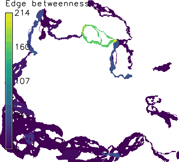
Figure: Corridors computed for connections on the minimum spanning tree weighted by edge betweenness in the example above.
r.connectivity.corridors loops through the user-selected edges (where option) of the edge-measure output vector map from r.connectivity.network and computes the respective corridor(s).
Corridors are defined as all pixels that have a lower average cost distance from a pair of patches, than the average cost distance between that pair. The user can add a tolerance for allowed deviation from cost distance within corridors in %, using the corridor_tolerance option.
r.connectivity.corridors can account for the importance of the corridors for the entire network by weighting them with regards to one or more network measures from r.connectivity.network, using the weights option.
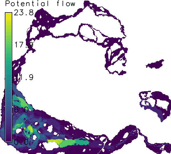
Thus, r.connectivity.corridors produces two types of output, that are named according to a user defined prefix and suffix:Finally, all individual corridors are being put together using r.series. In this step, the values of the cells in all corridor maps are summed up, which indicates the importance of an area (raster cell) for the network of the given patches (either the number of corridors a cell is part of, or other graph-theoretical measures for corridor importance).
In this example two alternative (or to some extent complementary) sets of corridors are calculated:
r.connectivity.corridors input=hws_connectivity_edge_measures layer=1 \
weights=cd_eb_ud suffix=mst corridor_tolerance=0.05 where="cf_mst_ud>0" \
cores=1
r.connectivity.corridors input=hws_connectivity_edge_measures layer=1 \
weights=cf_u suffix=all corridor_tolerance=0.05 \
cores=1
# Add the f-lag (-f) to the following two commands if you are sure you
# want to delete all intermediate maps from r.connectivity.*.
g.remove type=raster pattern=hws_connectivity_corridor_*
g.remove type=raster pattern=hws_connectivity_patch_*
Last changed: $Date$