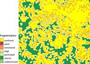
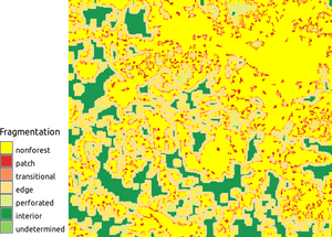
Two forest fragmentation indices with window size 7 (left) and 11 (right) show how increasing window size increases the amount of edges.
It follows a "sliding window" algorithm with overlapping windows. The amount of forest and its occurence as adjacent forest pixels within fixed- area "moving-windows" surrounding each forest pixel is measured. The window size is user-defined. The result is stored at the location of the center pixel. Thus, a pixel value in the derived map refers to "between-pixel" fragmentation around the corresponding forest location.
As input it requires a binary map with (1) forest and (0) non-forest. Obviously, one can replace forest any other land cover type. If one wants to exclude the influence of a specific land cover type, e.g., water bodies, it should be classified as no-data (NA) in the input map. See e.g., blog post.
Let Pf be the proportion of pixels in the window that are forested. Define Pff (strictly) as the proportion of all adjacent (cardinal directions only) pixel pairs that include at least one forest pixel, for which both pixels are forested. Pff thus (roughly) estimates the conditional probability that, given a pixel of forest, its neighbor is also forest. The classification model then identifies six fragmentation categories as:
interior:       Pf = 1.0
patch:          Pf < 0.4
transitional:   0.4 ≤ Pf < 0.6
edge:           Pf ≥ 0.6 and Pf - Pff < 0
perforated:     Pf ≥ 0.6 and Pf - Pff > 0
undetermined:   Pf ≥ 0.6 and Pf = Pff
g.region raster=landclass96
r.mapcalc "forest = if(landclass96 == 5, 1, 0)"
r.forestfrag input=forest output=fragmentation window=7
Two forest fragmentation indices with window size 7 (left) and 11 (right) show how increasing window size increases the amount of edges.
The addon is based on the r.forestfrag.sh script, with as extra options user-defined moving window size, option to trim the region (by default it respects the region) and a better handling of no-data cells.
Last changed: $Date$