DESCRIPTION

r.green.hydro.technical calculates the hydropower potential considering technical constrains that include head losses, efficiencies of the turbine, the shaft, the alternator and the transformer.

The input is a vector map with the intakes and restitutions of the potential plants as the one computed by r.green.hydro.recommended. The output is a vector map with the structure (derivation channel and penstock) for each potential plant with the value of the corrected power including these technical constrains.

NOTES

Firstly, the module computes the structure. As the current potential concerns especially small hydropower (inferior to 20 MW), the structure suggested is the one for small hydropower detailed in the picture below. It is composed of an intake (A) which diverts water from the river. This water is conveyed into a derivation channel (B) with a very low slope and arrives in a forebay tank (C) which regulates the fluctuation of discharge. Finally, the penstock (D) conveys the water with the highest possible head to the turbine-alternator group (E) which produces electricity. The water is then released into the river (restitution F). We use the following vocabulary: the structure of the plant corresponds to the part with the derivation channel, the forebay tank and the penstock, whereas the segment of the plant corresponds to the part of the river (water not diverted) between the intake (A) and the restitution (F).

structure
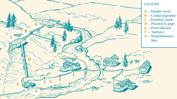
Structure of the plants considered in the module


The power is maximized for the highest head in the penstock so the derivation channel is computed along the same quote (the low slope is neglected here) until the point which maximizes the head along the penstock. The structure is computed for both sides of the river in order to determine which one produces the most power.

Using the computed structure, the module calculates the head losses:

- in the derivation channel
There are regular losses calculated thanks to Manning's formula: Δhderiv=L*(Q/(ks*A*Rh2/3))2
where Rh is the hydraulic radius (m),
A the cross sectional area of flow (m2),
L is the channel length (m),
Q is the discharge (m3/s),
ks the Strickler coefficient (m1/3/s), we consider steel as default parameter, with ks=75 m1/3/s.

- in the forebay tank
There are singular losses caused by the change of section in the forebay tank and the change of direction in the penstock (steep slope).
In any case, singular head losses are expressed like this: Δhsing=K*V2/(2g)
where V is the velocity (m/s),
g the gravity term (9,81 m/s2),
K is a coefficient determined according to the kind of singularity.
In our case, the singular losses are the sum of the ones for these three phenomena:
- enlargement at the entrance of the forebay tank: K1=1 and V=1 m/s
- narrowing at the exit of the forebay tank: K2=0.5 and V=4Q/(πD2) m/s
- bend at the beginning of the penstock: K3=(gross head/L)2+2*sin(ASIN(gross head/L)/2)4 and V=4Q/(πD2) m/s

- in the penstock
There are regular losses calculated thanks to this formula: Δhpen=(f*8*L*Q2)/(π2*D5*g)
where L is the penstock length (m),
D is the penstock diameter (m),
Q is the discharge (m3/s),
f is the Darcy-Weisbach friction coefficient, which can be determined by Colebrooke formula. We consider steel by default with absolute roughness of ε = 0,015 mm.

Then, the module chooses the turbine which is the most accurate for each plant. The data of possible turbines of which you have to enter the path into the turbine_folder=string field, are gathered in the folder turbine. For each turbine there is a text file with the ranges of discharge and head required to use it. There is also the efficiency in function of QW/Q_design. The turbine is designed to work at Q_design and QW corresponds to the real discharge which flows in the turbine. As we don't consider the duration curves but only the mean annual discharge, we assume that QW=Q_design.

If you want to create an additional text file for another turbine model, the file has to have this scheme with the correct information at the corresponding lines:
TURBINE 	           ALPHA_C
Name of the turbine	   Value of alpha_c
Q_MIN		           Q_MAX
Value of q_min	           Value of q_max
DH_MIN		           DH_MAX
Value of dh_min	           Value of dh_max
QW/Q_design	           ETA
Coordinates of the curve efficiency=f(QW/Q_design)

In the turbine folder there is already the text file called list with a large choice of turbines available. You have to enter the path of the list file into the turbine_list=string field of the GUI. But the user can also create his own text file that has to have the same structure with a list of the names of the turbines he has selected and wants to be considered.

To choose the turbine, the module first selects the turbines with ranges of discharge and head containing the values of the corresponding potential plant. Among these turbines, it chooses the one which has the best efficiency for QW=Q_design.

Thus the efficiency of the turbine is found. The global efficiency also includes the efficiencies of the shaft, the alternator and the transformer which can be chosen or they are respectively equal to 1, 0.96 and 0.99 by default.

Finally, the corrected value of power which can be exploited is calculated.
It corresponds to P=η*ρ*g*Q*Δhnet
where η is the global efficiency of the plant (turbine, shaft, alternator and transformer),
ρ the density of water (1000 kg/m3),
g the gravity term (9,81 m/s2),
Q the discharge (m3/s),
Δhnet the net head, that means the gross head minus head losses

The output map of the module is the one with the structure for each plant, including in the table the data of:
- discharge (m3/s)
- gross head (m)
- kind of the channel: derivation (conduct) or penstock
- side of the river (option0 or option1)
- diameter of the channel (m)
- losses in the channel (m)

Moreover, only in the penstock's line of the structure, there are:
- singular losses (m) in the forebay tank between the derivation channel and the penstock
- the total losses (m) for each structure, which are the sum of the regular losses in the derivation channel and in the penstock and the singular losses in the forebay tank
- net head (m), which is the gross head minus the total losses
- hydraulic power (hyd_power, in kW) which is the power considering the gross head and a global efficiency equal to 1. It corresponds to the theoretical power (the maximum)
- efficiency of the selected turbine (e_turbine)
- kind of the selected turbine (turbine)
- power (kW) which can be exploited considering the technical constrains
- global efficiency (power/hyd_power)
- max_power: yes or no, yes for the side (option1 or option0) which produces the most power

EXAMPLE

This example is based on the case-study of Gesso and Vermenagna valleys in the Natural Park of the Maritime Alps, Piedmont, Italy.

Here is the input vector map potentialplants with the intakes and restitutions (in red) computed by r.green.hydro.recommended. The vector map with the segments of river is also visible in blue in this picture. These potential plants have a maximum length of 800 m and a distance of 800 m between them.
input
Potential intakes and restitutions


The following command that you can either put in the command console or the GUI of r.green.hydro.technical computes the structure of the potential plants for each side of the river and includes the corrected power on the output map table:
r.green.hydro.technical plant=potentialplants elevation=elevation output_struct=techplants output_plant=segmentplants
turbine_folder=/pathtothefileoftheturbine_folder  turbine_list=/pathtothefileoftheturbine_list

The result is shown in the following vector map called techplants. The table of this map is completed as explained in the end of the NOTES part.

output
Structure of the potential plants in black (techplants map)


SEE ALSO

r.green.hydro.discharge
r.green.hydro.delplants
r.green.hydro.theoretical
r.green.hydro.recommended
r.green.hydro.structure
r.green.hydro.optimal
r.green.hydro.financial

REFERENCE

Picture of the plant structure taken from Micro-hydropower Systems - A Buyer's Guide, Natural Resources Canada, 2004
Sources for the theory : Courses of French engineering schools ENSE3 Grenoble-INP (Hydraulique des ecoulements en charge) and ENGEES Strasbourg (Hydraulique a surface libre)

AUTHORS

Giulia Garegnani (Eurac Research, Bolzano, Italy), Julie Gros (Eurac Research, Bolzano, Italy), Manual written by Julie Gros.
Last changed: $Date : 2015-06-12 15:46 GMT+1$