DESCRIPTION

r.learn.ml represents a front-end to the scikit learn python package. The module enables scikit-learn classification and regression models to be applied to GRASS GIS rasters that are stored as part of an imagery group group or specified as individual maps in the optional raster parameter. Several commonly used classifiers and regressors are exposed in the GUI and the choice of classifier is set using the classifier parameter. For more details relating to the classifiers, refer to the scikit learn documentation. The following classification and regression methods are available:

• LogisticRegression represents a linear model for classification and is a modification of linear regression, but using the logistic distribution which enables the use of a categorical response variable. If the response raster is coded to 0 and 1, then a binary classification occurs, but the scikit-learn logistic regression can also perform a multiclass classification using a one-versus-rest scheme.
• LinearDiscriminantAnalysis and QuadraticDiscriminantAnalysis are classifiers with linear and quadratic decision surfaces. These classifiers do not take any parameters and are inherently multiclass. They can only be used for classification.
• KNeighborsClassifier classifies samples based on closest distance to a predefined number of training samples. Two hyperparameters are exposed, with n_neighbors governing the number of neighbors to use to decide the prediction label, and weights specifying whether these neighbors should have equal weights or whether they should be inversely weighted by their distance.
• GaussianNB is the Gaussian Naive Bayes algorithm and can be used for classification only. Naive Bayes is a supervised learning algorithm based on applying Bayes theorem with the naive assumption of independence between every pair of features. This classifier does not take any parameters.
• The DecisionTreeClassifier and DecisionTreeRegressor map observations to a response variable using a hierarchy of splits and branches. The terminus of these branches, termed leaves, represent the prediction of the response variable. Decision trees are non-parametric and can model non-linear relationships between a response and predictor variables, and are insensitive the scaling of the predictors.
• The RandomForestsClassifier and RandomForestsRegressor represent ensemble classification and regression tree methods. Random forests overcome some of the disadvantages of single decision trees by constructing an ensemble of uncorrelated trees. Each tree is constructed from a random subsample of the training data and only a random subset of the predictors based on max_features is made available during each node split. Each tree produces a prediction probability and the final classification result is obtained by averaging of the prediction probabilities across all of the trees. The ExtraTreesClassifier is a variant on random forests where during each node split, the splitting rule that is selected is based on the best of a collection of randomly-geneated thresholds that were assigned to the features.
• The GradientBoostingClassifier and GradientBoostingRegressor also represent ensemble tree-based methods. However, in a boosted model the learning processes is additive in a forward step-wise fashion whereby n_estimators are fit during each model step, and each model step is designed to better fit samples that are not currently well predicted by the previous step. This incrementally improves the performance of the entire model ensemble by fitting to the model residuals. Additionally, Microsoft's LGBMClassifier and LGBMRegressor models represent an accelerated version of gradient boosting which can optionally be installed by pip install lightgbm.
• The SVC model is C-Support Vector Classifier. Only a linear kernel is supported because non-linear kernels using scikit learn for typical remote sensing and spatial analysis datasets which consist of large numbers of samples are too slow to be practical. This classifier can still be slow for large datasets that include > 10000 training samples.
• The EarthClassifier and EarthRegressor is a python-based version of Friedman's multivariate adaptive regression splines. This classifier depends on the py-earth package, which optionally can be installed in addition to scikit-learn. Earth represents a non-parametric extension to linear models such as logistic regression which improves model fit by partitioning the data into subregions, with each region being fitted by a separate regression term.

The Classifier parameters tab provides access to the most pertinent parameters that affect the previously described algorithms. The scikit-learn classifier defaults are generally supplied, and some of these parameters can be tuning using a grid-search by inputting multiple parameter settings as a comma-separated list. This tuning can also be accomplished simultaneously with nested cross-validation by also settings the cv option to > 1. The parameters consist of:

• C is the inverse of the regularization strength, which is when a penalty is applied to avoid overfitting. C applies to the LogisticRegression and SVC models.
• n_estimators represents the number of trees in Random Forest model, and the number of trees used in each model step during Gradient Boosting. For random forests, a larger number of trees will never adversely affect accuracy although this is at the expensive of computational performance. In contrast, Gradient boosting will start to overfit if n_estimators is too high, which will reduce model accuracy.
• max_features controls the number of variables that are allowed to be chosen from at each node split in the tree-based models, and can be considered to control the degree of correlation between the trees in ensemble tree methods.
• min_samples_split and min_samples_leaf control the number of samples required to split a node or form a leaf node, respectively.
• The learning_rate and subsample parameters apply only to Gradient Boosting. learning_rate shrinks the contribution of each tree, and subsample is the fraction of randomly selected samples for each tree. A lower learning_rate always improves accuracy in gradient boosting but will require a much larger n_estimators setting which will lower computational performance.
• The main control on accuracy in the Earth classifier consists max_degree which is the maximum degree of terms generated by the forward pass. Settings of max_degree = 1 or 2 offer good accuracy versus computational performance.

In addition to model fitting and prediction, feature selection can be performed using the -f flag. The feature selection method employed is based on Brenning et al. (2012) and consists of a custom permutation-based method that can be applied to all of the classifiers as part of a cross-validation. The method consists of: (1) determining a performance metric on a test partition of the data; (2) permuting each variable and assessing the difference in performance between the original and permutation; (3) repeating step 2 for n_permutations; (4) averaging the results. Steps 1-4 are repeated on each k partition. The feature importance represent the average decrease in performance of each variable when permuted. For binary classifications, the AUC is used as the metric. Multiclass classifications use accuracy, and regressions use R2.

Cross validation can be performed by setting the cv parameters to > 1. Cross-validation is performed using stratified kfolds, and multiple global and per-class accuracy measures are produced depending on whether the response variable is binary or multiclass, or the classifier is for regression or classification. The cvtype parameter can also be changed from 'non-spatial' to either 'clumped' or 'kmeans' to perform spatial cross-validation. Clumped spatial cross-validation is used if the training pixels represent polygons, and then cross-validation will be effectively performed on a polygon basis. Kmeans spatial cross-validation will partition the training pixels into n_partitions by kmeans clustering of the pixel coordinates. These partitions will then be used for cross-validation, which should provide more realistic performance measures if the data are spatially correlated. If these partioning schemes are not sufficient then a raster containing the group_ids of the partitions can be supplied using the group_raster option.

Although tree-based classifiers are insensitive to the scaling of the input data, other classifiers such as linear models may not perform optimally if some predictors have variances that are orders of magnitude larger than others. The -s flag adds a standardization preprocessing step to the classification and prediction to reduce this effect. Additionally, most of the classifiers do not perform well if there is a large class imbalance in the training data. Using the -b flag balances the training data by weighting of the minority classes relative to the majority class. This does not apply to the Naive Bayes or LinearDiscriminantAnalysis classifiers.

Non-ordinal, categorical predictors are also not specifically recognized by scikit-learn. Some classifiers are not very sensitive to this (i.e. decision trees) but generally, categorical predictors need to be converted to a suite of binary using onehot encoding (i.e. where each value in a categorical raster is parsed into a separate binary grid). Entering the indices (comma-separated) of the categorical rasters as they are listed in the imagery group as 0...n in the categorymaps option will cause onehot encoding to be performed on the fly during training and prediction. The feature importances are returned as per the original imagery group and represent the sum of the feature importances of the onehot-encoded variables. Note: it is important that the training samples all of the categories in the rasters, otherwise the onehot-encoding will fail when it comes to the prediction.

The module also offers the ability to save and load a classification or regression model (save_model=name[.gz]). Note that the model file size can become quite large; when using a supported filename extensions (incl. '.gz', '.bz2', '.xz' or '.lzma') the model file will be automatically compressed. Saving and loading a model allows a model to be fitted on one imagery group, with the prediction applied to additional imagery groups. This approach is commonly employed in species distribution or landslide susceptibility modelling whereby a classification or regression model is built with one set of predictors (e.g. present-day climatic variables) and then predictions can be performed on other imagery groups containing forecasted climatic variables.

For convenience when performing repeated classifications using different classifiers or parameters, the training data can be saved to a csv file using the save_training option. This data can then be loaded into subsequent classification runs, saving time by avoiding the need to repeatedly query the predictors.

NOTES

r.learn.ml uses the "scikit-learn" machine learning python package along with the "pandas" package. These packages need to be installed within your GRASS GIS Python environment. For Linux users, these packages should be available through the linux package manager. For MS-Windows users using a 64 bit GRASS, the easiest way of installing the packages is by using the precompiled binaries from Christoph Gohlke and by using the OSGeo4W installation method of GRASS, where the python setuptools can also be installed. You can then use 'easy_install pip' to install the pip package manager. Then, you can download the NumPy+MKL and scikit-learn .whl files and install them using 'pip install packagename.whl'. For MS-Windows with a 32 bit GRASS, scikit-learn is available in the OSGeo4W installer.

r.learn.ml is designed to keep system memory requirements relatively low. For this purpose, the rasters are read from the disk row-by-row, using the RasterRow method in PyGRASS. This however does not represent an efficient volume of data to pass to the classifiers, which are mostly multithreaded. Therefore, groups of rows specified by the rowincr parameter are passed to the classifier, and the reclassified image is reconstructed and written row-by-row back to the disk. rowincr=25 should be reasonable for most systems with 4-8 GB of ram. The row-by-row access however results in slow performance when sampling the imagery group to build the training data set when providing a raster as the trainingmap. Instead, the default behaviour is to read each predictor into memory at a time. If this still exceeds the system memory then the -l flag can be set to write each predictor to a numpy memmap file, and classification/regression can then be performed on rasters of any size irrespective of the available memory.

Many of the classifiers involve a random process which can causes a small amount of variation in the classification results, out-of-bag error, and feature importances. To enable reproducible results, a seed is supplied to the classifier. This can be changed using the randst parameter.

EXAMPLE

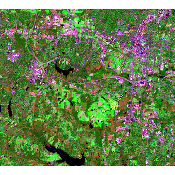
Here we are going to use the GRASS GIS sample North Carolina data set as a basis to perform a landsat classification. We are going to classify a Landsat 7 scene from 2000, using training information from an older (1996) land cover dataset.

Landsat 7 (2000) bands 7,4,2 color composite example:

Note that this example must be run in the "landsat" mapset of the North Carolina sample data set location.

First, we are going to generate some training pixels from an older (1996) land cover classification:

g.region raster=landclass96 -p
r.random input=landclass96 npoints=1000 raster=landclass96_roi

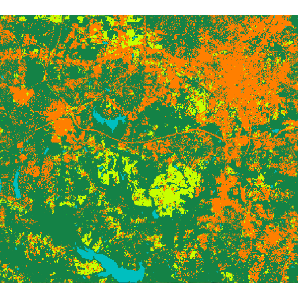
Then we can use these training pixels to perform a classification on the more recently obtained landsat 7 image:

r.learn.ml group=lsat7_2000 trainingmap=landclass96_roi output=rf_classification \
  classifier=RandomForestClassifier n_estimators=500
# copy category labels from landclass training map to result
r.category rf_classification raster=landclass96_roi
# copy color scheme from landclass training map to result
r.colors rf_classification raster=landclass96_roi
r.category rf_classification

Random forest classification result:

ACKNOWLEDGEMENTS

Thanks for Paulo van Breugel and Vaclav Petras for testing.

REFERENCES

Brenning, A. 2012. Spatial cross-validation and bootstrap for the assessment of prediction rules in remote sensing: the R package 'sperrorest'. 2012 IEEE International Geoscience and Remote Sensing Symposium (IGARSS), 23-27 July 2012, p. 5372-5375.

Scikit-learn: Machine Learning in Python, Pedregosa et al., JMLR 12, pp. 2825-2830, 2011.

AUTHOR

Last changed: $Date$