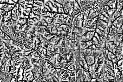
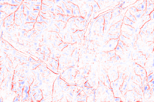
Figure: Local relief model of downtown Raleigh area created from elevation raster map in NC sample location with the default (gray scale) color table and custom red (negative values) and blue (positive values) color table
r.local.relief generates a local relief model (LRM) from lidar-derived high-resolution DEMs. Local relief models enhance the visibility of small-scale surface features by removing large-scale landforms from the DEM.
Generating the LRM is accomplished in 7 steps (Hesse 2010:69):
The interpolation step is performed by the r.fillnulls module by default (using cubic interpolation). If this is not working on your data, you can use -v flag to use v.surf.bspline cubic interpolation instead (this might be slower on some types of data).
The final local relief model is named according to the output parameter. When the -i flag is specified, r.local.relief creates additional output files representing the intermediate steps in the LRM generation process. The names and number of the intermediate files vary depending on whether r.fillnulls (default) or v.surf.bspline (specified by using the -v flag) is used for interpolation. The intermediate maps are composed of the user-specified output parameter and suffixes describing the intermediate map.
Without using the -v flag (r.fillnulls interpolation), intermediate maps have the following suffixes:
With using the -v flag (v.surf.bspline interpolation), intermediate maps have the following suffixes:
The module sets equalized gray scale color table for local relief model map and for the elevation difference (subtracted elevations). The color tables of other raster maps are set to the same color table as the input elevation map has.
r.local.relief input=elevation output=lrm11
r.local.relief input=elevation output=lrm25 neighborhood_size=25
r.local.relief -i input=elevation output=lrm11
r.local.relief -i -v input=elevation output=lrm11
# set the computational region to area of interest
g.region n=228010 s=223380 w=637980 e=644920 res=10

# compute local relief model
r.local.relief input=elevation output=elevation_lrm

# show the maps, e.g. using monitors
d.mon wx0
d.rast elevation
d.rast elevation_lrm

# try alternative red (negative values) and blue (positive values) color table
# color table shows only the high values which hides small streets
# for non-unix operating systems use file or interactive input in GUI
# instead of rules=- and EOF syntax
r.colors map=elevation_lrm@PERMANENT rules=- <<EOF
100% 0:0:255
0 255:255:255
0% 255:0:0
nv 255:255:255
default 255:255:255
EOF
Figure: Local relief model of downtown Raleigh area created from elevation raster map in NC sample location with the default (gray scale) color table and custom red (negative values) and blue (positive values) color table
Vaclav Petras, NCSU OSGeoREL,
Eric Goddard
Last changed: $Date$