DESCRIPTION
r.series.lwr performs a local weighted regression (LWR,
Cleveland and Devlin 1988) of time series in order to estimate missing
values and identify outliers. For each input map, an output map with
the suffix suffix (default: _lwr) is created.
For each observation in the time series, the (in time) neighboring
values are used to estimate a polynomial function that best fits the
observations. The values are weighted according to their distance (in
time) to the current observation. Values that are farther away in time
get lower weights. The main difference among the different
weight funtions lies in how strongly the current observation is
emphasized with respect to its temporal neighbors. See this dedicated
wiki
for further details.
The option order determines the order of the polynomial function
used to fit the observations. An order of 0 is a weighted average, an
order of 1 is a linear regression. Recommended and default is
order=2. An order of 3 might cause over-fitting, resulting in
no smoothing, and should only be used with data that show high
fluctuations.
The delta option is experimental. It smoothes the polynomial
function. With a high delta value, a higher order polynomial
function fitting becomes similar to a moving average.
Optionally, low and/or high outliers can be removed when fitting a
polynomial by means of the -l and -h flags,
respectively. In this case, a fit error tolerance (option fet)
must be provided. The value of fet is relative to the value range of the
variable being considered.
The use of these flags will slow down the module and they are only
needed when the time series contains many outliers. A few outliers are
handled well with the default settings.
All gaps in the time series are by default interpolated, as long as the
time series contains sufficient non-NULL observations. Optionally, the
maximum size of gaps to be interpolated can be set with the
maxgap option. The units of maxgap are the units of the time
steps.
Extrapolation can be avoided with the -i flag. In this case,
LWR is performed only from the first to the last non-NULL observation
in the time series.
The module uses an adaptive bandwidth to fit the polynomial and
searches for order + 1 + dod valid values around the current
observation. The degree of over-determination (dod) is the user defined
number of extra temporal neighbours that should be considered for the
estimation of the value at each time step.
There is a trade-off between the goodness of fit to existing/original
data and avoiding overshoots in gaps. This trade-off can be observed in
the example below when order=2 is used along with dod=0.
In this case, the reconstruction will most of the time be an exact match
to the input data because LWR will try to copy the slopes in the data,
including those very steep slopes, but this might create overshootings
in gaps. The risk of overshootings can be alleviated by increasing dod
(i.e. dod > 0), which will smooth the output. The effect of a dod=5 can
be observed in the examples below.
NOTES
If the range option is given, all the values falling outside
the low,high thresholds will be treated as if they were NULL.
The low,high thresholds are floating point. Therefore, use
-inf or inf for a single threshold (e.g.,
range=0,inf to ignore negative values, or
range=-inf,-200.4 to ignore values above -200.4).
There is no need to give time steps if the time interval among maps is
constant. If the interval is not constant, the user needs to assign time
steps. These must always increase (i.e.: each time step must be larger
than the previous one) and the total number of time steps must be equal
to the number of input maps.
The maximum number of raster maps that can be processed is given by the
user-specific limit of the operating system. For example, the soft limits
for users are typically 1024. The soft limit can be changed with e.g.
ulimit -n 4096 (UNIX-based operating systems) but it cannot be
higher than the hard limit. If the latter is too low, you can as superuser
add an entry in:
/etc/security/limits.conf
# <domain>      <type>  <item>         <value>
your_username  hard    nofile          4096
cat /proc/sys/fs/file-max
Use the -z flag to analyze large amounts of raster maps without
hitting open files limit and the file option to avoid hitting
the size limit of command line arguments.
Note that the computation using the file option is slower than
with the input option.
For every single row in the output map(s) all input maps are opened and
closed. The amount of RAM will rise linearly with the number of
specified input maps. The input and file options are
mutually exclusive: the former is a comma separated list of raster map
names and the latter is a text file with a new line separated list of
raster map names. Note that the order of maps in one option or
the other is very important.
EXAMPLES
We use a time series of the Chlorophyll-a concentration level 3 product
from MODIS Aqua (spatial resolution approx. 4 km and temporal
resolution 8 days) to exemplify different parameter settings in
r.series.lwr. We will first execute the module with default options to
interpolate all existent gaps with a polynomial of first order (i.e.
order=1). Second, we change to a second order polynomial (i.e.
order=2). The third case shows how to use -l/-h flags in
combination with fet to remove outliers. In this example we
will remove only high outiliers (-h flag) and we set a value of fet
relative to the values of Chlorophyll-a concentration. The fourth
example demonstrates the use of dod to consider more time
steps when fitting the polynomial at each observation (Note that the
resulting series is smoother, i.e. the fluctuations have been
smoothed). Finally, we set a value for maxgap, so that only
temporal gaps equal to or smaller than the maximum gap will be
interpolated.
# list of maps
maplist=`g.list type=raster pattern=A201[2-3]*chlor_a* sep=,`

# 1. default settings (order=1)
r.series.lwr input=$maplist suffix=_lwr1 order=1 weight=tricube

# 2. change to order=2
r.series.lwr input=$maplist suffix=_lwr2 order=2 weight=tricube

# 3. set degree of overdetermination (dod) to consider more time steps (smoothes the series)
r.series.lwr -i input=$maplist suffix=_lwr3 order=2 weight=tricube dod=5

# 4. set dod > 1 and -h flag to identify and remove high outliers with fit error tolerance (fet=0.5)
r.series.lwr -i -h input=$maplist suffix=_lwr4 order=2 weight=tricube dod=5 fet=0.5

# 5. set maxgap (temporal gaps longer than maxgap will not be filled)
r.series.lwr -i input=$maplist suffix=_lwr5 order=2 weight=tricube maxgap=4
for i in `seq 1 5` ; do

 # create time series with lwr outputs
 t.create type=strds temporaltype=absolute output=cla_lwr${i} \
  title="LWR output for Chl-a" \
  description="MODIS Aqua L3 Chl-a 8-day 4km 2012-2013. Reconstruction with r.series.lwr - run ${i}"

 # create list with filenames to parse
 g.list type=raster pattern="*_lwr${i}" output=names_list_${i}

 # parse filenames, convert YYYYDOY to YYYY-MM-DD and write file to use in t.register
 for mapname in `cat names_list_${i}` ; do
  year_start=`echo ${mapname:1:4}`
  doy_start=`echo ${mapname:5:3}`
  year_end=`echo ${mapname:8:4}`
  doy_end=`echo ${mapname:12:3}`

  # convert YYYY-DOY to YYYY-MM-DD
  doy_start=`echo "$doy_start" | sed 's/^0*//'`
  doy_end=`echo "$doy_end" | sed 's/^0*//'`
  START_DATE=`date -d "${year_start}-01-01 +$(( ${doy_start} - 1 ))days" +%Y-%m-%d`
  END_DATE=`date -d "${year_end}-01-01 +$(( ${doy_end} ))days" +%Y-%m-%d`

  # print mapname, start and end date
  echo "$mapname|$START_DATE|$END_DATE" >> map_list_start_and_end_time_${i}.txt
 done

 # register maps in strds
 t.register input=cla_lwr${i} type=raster file=map_list_start_and_end_time_${i}.txt

 # get info
 t.info cla_lwr${i}

done
g.gui.tplot strds=cla_2012_2013 coordinates=-61.196485623,-45.3232161874
g.gui.tplot strds=cla_lwr1,cla_lwr2 coordinates=-61.196485623,-45.3232161874
g.gui.tplot strds=cla_lwr3,cla_lwr4 coordinates=-61.196485623,-45.3232161874
g.gui.tplot strds=cla_lwr5,cla_2012_2013 coordinates=-61.196485623,-45.3232161874
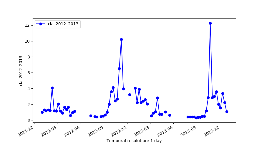 Original series (cla_2012_2013)
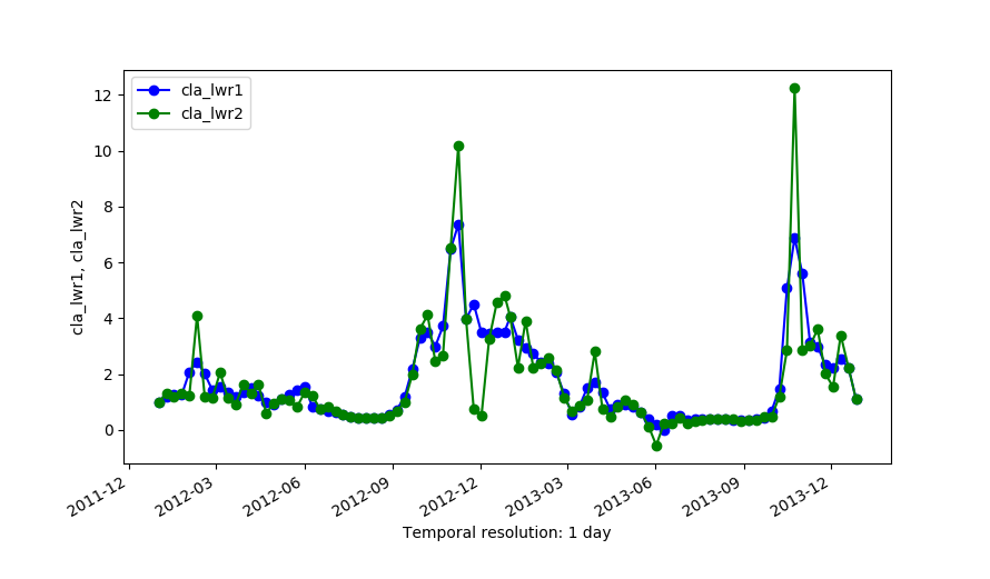 Outputs of LWR with order=1 (cla_lwr1) and order=2 (cla_lwr2).
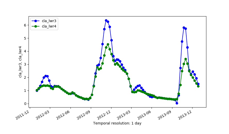 Outputs of LWR with dod=5 (cla_lwr3) and dod=5 plus -h flag and fet=0.5 (cla_lwr4).
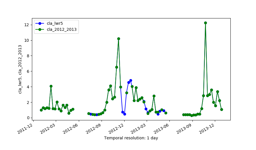 Original series (cla_2012_2013) and the output of LWR with maxgap=4 (cla_lwr5).
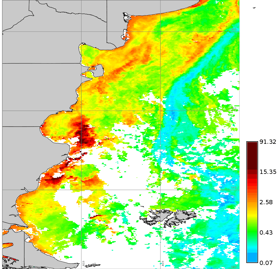
 Comparison of an original Chlorophyll-a map and a reconstructed map (dod=5).
REFERENCES
Cleveland, William S.; Devlin, Susan J. (1988). Locally-Weighted
Regression: An Approach to Regression Analysis by Local Fitting,
Journal of the American Statistical Association, 83 (403), 596-610,
doi:10.2307/2289282
SEE ALSO
r.series,
r.hants
Temporal data processing Wiki
AUTHOR
Markus Metz
Last changed: $Date$