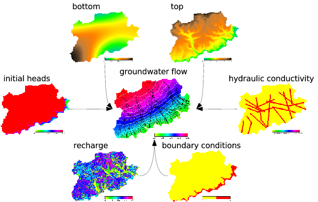
r.gwflow calculates the piezometric head and optionally the
filter velocity field, based on the hydraulic conductivity and the piezometric head.
The vector components can be visualized with paraview if they are exported
with r.out.vtk.
The groundwater flow will always be calculated transient.
If you want to calculate stady state, set the timestep
to a large number (billions of seconds) or set the
specific yield/ effective porosity raster maps to zero.
(dh/dt)*Ss = Kxx * (d^2h/dx^2) + Kyy * (d^2h/dy^2) + q
# set the region accordingly
g.region res=25 res3=25 t=100 b=0 n=1000 s=0 w=0 e=1000

#now create the input raster maps for confined and unconfined aquifers
r.mapcalc "phead=if(row() == 1 , 50, 40)"
r.mapcalc "status=if(row() == 1 , 2, 1)"
r.mapcalc "well=if(row() == 20 && col() == 20 , -0.001, 0)"
r.mapcalc "hydcond=0.00025"
r.mapcalc "recharge=0"
r.mapcalc "top_conf=20.0"
r.mapcalc "top_unconf=70.0"
r.mapcalc "bottom=0.0"
r.mapcalc "null=0.0"
r.mapcalc "poros=0.15"
r.mapcalc "syield=0.0001"

#confined groundwater flow with cg solver and sparse matrix
r.gwflow --o -s solver=cg top=top_conf bottom=bottom phead=phead status=status \
hc_x=hydcond hc_y=hydcond q=well s=syield r=recharge output=gwresult_conf \
dt=8640000 type=confined velocity=gwresult_conf_velocity

#unconfined groundwater flow with cg solver and sparse matrix
r.gwflow --o -s solver=cg top=top_unconf bottom=bottom phead=phead \
status=status hc_x=hydcond hc_y=hydcond q=well s=poros r=recharge \
output=gwresult_unconf dt=8640000 type=unconfined velocity=gwresult_unconf_velocity

# The data can be visulaized with paraview when exported with r.out.vtk
r.out.vtk -p in=gwresult_conf,status vector=gwresult_conf_velocity_x,gwresult_conf_velocity_y,null out=/tmp/gwdata_conf2d.vtk
r.out.vtk -p elevation=gwresult_unconf in=gwresult_unconf,status vector=gwresult_unconf_velocity_x,gwresult_unconf_velocity_y,null out=/tmp/gwdata_unconf2d.vtk

#now load the data into paraview
paraview --data=/tmp/gwdata_conf2d.vtk &
paraview --data=/tmp/gwdata_unconf2d.vtk &
Last changed: $Date$