DESCRIPTION

The Graphical Modeler is a wxGUI component which allows the user to create, edit, and manage complex models using easy-to-use interface. When performing analytical operations in GRASS, the operations are not isolated, but part of a chain of operations. Using Graphical Modeler, that chain of processes (ie. GRASS modules) can be wrapped into one process (ie. model). So it's easier to execute the model later with slightly different inputs or parameters.
Models represent a programming technique used in GRASS GIS to concatenate models together to accomplish a task. It is advantageous when user see boxes and ovals that are connected by lines and represent some tasks rather than seeing lines of coded text. Graphical Modeler can be used as custom tool that automates a process. Created model can simplify or shorten a task can be run many times and it can also be shared with others. Important note is that models cannot perform specified tasks that one cannot perform manually with GRASS GIS. It is recommended to first do process manually, note the steps (eg. using Copy button in module dialogs) and later duplicate them in model.

The Graphical Modeler allows you to:

• define data items (raster, vector, 3D raster maps)
• define actions (GRASS commands)
• define relations between data and action items
• define loops (eg. map series) and conditions (if-else statements)
• define model variables
• parameterize GRASS commands
• define intermediate data
• validate and run model
• store model properties to the file (GRASS Model File|*.gxm)
• export model to Python script
• export model to image file

Main dialog

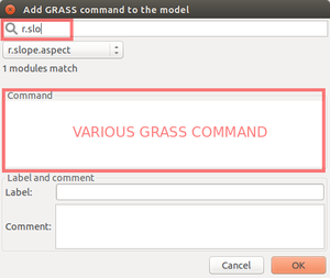
The main Graphical Modeler menu contains options which enable the user to fully control the model. Directly under the main menu one can find toolbar with buttons (see figure below). There are options like (1) Create new model, (2) Load model from file, (3) Save current model to file, (4) Export model to image, (5) Export model to Python script, (6) Add command (GRASS modul) to model, (7) Add data to model, (8) Manually define relation between data and commands, (9) Add loop/series to model, (10) Add comment to model, (11) Redraw model canvas, (12) Validate model, (13) Run model, (14) Manage model variables, (15) Model settings, (16) Show manual and last of them is button (17) Quit Graphical Modeler.

Figure: Components of Graphical Modeler menu toolbar.

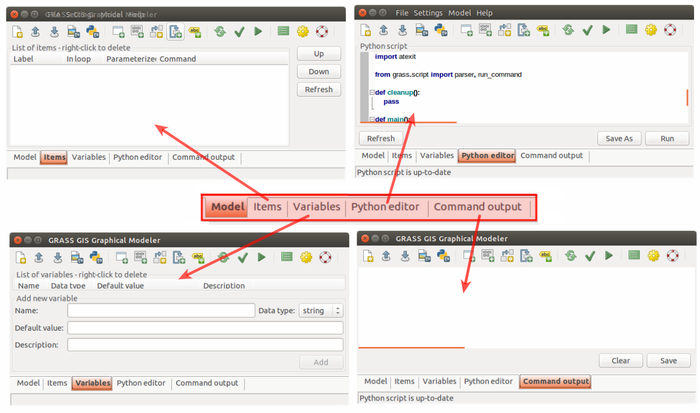
There is also lower menu bar in Graphical modeler dialog where one can manage model items, see commands, add or manage model variables, define default values and descriptions. Python editor dialog window allows seeing performation written in Python code. Rightmost tab of bottom menu is automatically triggered when model is activated and shows all the steps of running GRASS modeler modules. In case of some errors in calculation process, it is written at that place.

Figure: Lower Graphical Modeler menu toolbar.

Components of models

• (A) raster data:
• (B) relation:
• (C) GRASS module:
• (D) loop:
• (E) database table:
• (F) 3D raster data:
• (G) vector data:
• (H) disabled GRASS module:
• (I) comment:

Figure: A model to perform unsupervised classification using MLC (i.maxlik) and SMAP (i.smap).

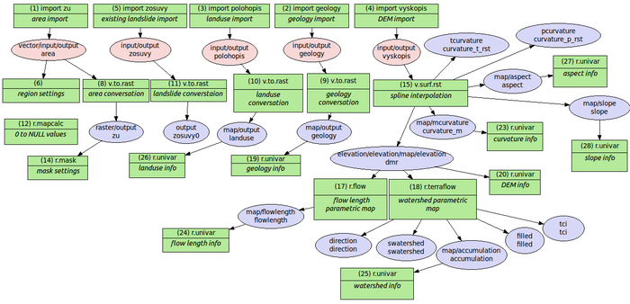
Another example:

Figure: A model to perform estimation of average annual soil loss caused by sheet and rill erosion using The Universal Soil Loss Equation.

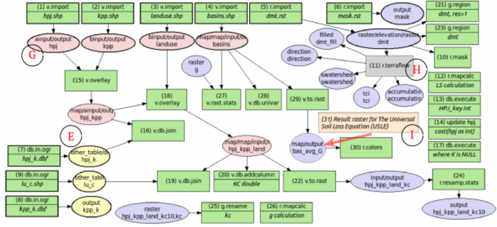
Example as part of landslide prediction process:

Figure: A model to perform creation of parametric maps used by geologists to predict landlides in area of interest.

EXAMPLE

In command console it would be as follows:

# input data import
r.import input=elev_state_500m.tif output=elevation 
v.import input=zipcodes_wake.shp output=zipcodes_wake 
# computation region settings
g.region vector=zipcodes_wake  
# raster statistics (average values), upload to vector map table calculation
v.rast.stats -c map=zipcodes_wake raster=elevation column_prefix=rst method=average 
# univariate statistics on selected table column for zipcode map calculation
v.db.univar map=zipcodes_wake column=rst_average 
# conversation from vector to raster layer (due to result presentation)
v.to.rast input=zipcodes_wake output=zipcodes_avg use=attr attribute_column=rst_average 
# display settings
r.colors -e map=zipcodes_avg color=bgyr                                         
d.mon start=wx0 bgcolor=white                                                   
d.barscale style=arrow_ends color=black bgcolor=white fontsize=10
d.rast map=zipcodes_avg bgcolor=white                                                                                                 
d.vect map=zipcodes_wake type=boundary color=black                                                     
d.northarrow style=1a at=85.0,15.0 color=black fill_color=black width=0 fontsize=10
d.legend raster=zipcodes_avg lines=50 thin=5 labelnum=5 color=black fontsize=10 

Figure: Dialog for adding GRASS commands to model.

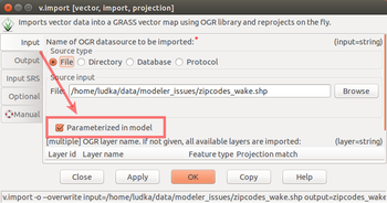
All of used modules can be parameterized in model. That causes launching dialog with input options for model after model is run. In this example input layers (zipcodes_wake vector data and elev_state_500m raster data) are parameterized. Parameterized elements have a little thicker boarder in model scheme with diagrams.

Figure: A model parameter settings.

Final model, list of all model items, Python code window with Save and Run option are on figures below.

Figure: A model to perform average statistics for zipcode zones.

Figure: Items with Python editor window.

The resultant model for Graphical Modeler is available here.

After model is run with button and inputs are set, results can be displayed as follows:

Figure: Average elevation for zipcodes using North Carolina sample dataset as automatic calculation performed by Graphical Modeler.

Very useful advantage is that for example, this model can later be used to calculate (let's say) average precipe value for every administrative region in Slovakia using precip raster data from Slovakia precipitation dataset and administration boundaries of Slovakia from Slovak Geoportal (only with a few clicks).

SEE ALSO

See also the wiki page (especially various video tutorials).

AUTHORS

$Date$