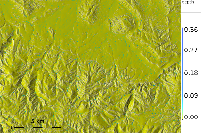
Figure: Water depth map in the Spearfish (SD) area
The module automatically converts horizontal distances from feet to metric system using database/projection information. Rainfall excess is defined as rainfall intensity - infiltration rate and should be provided in [mm/hr]. Rainfall intensities are usually available from meteorological stations. Infiltration rate depends on soil properties and land cover. It varies in space and time. For saturated soil and steady-state water flow it can be estimated using saturated hydraulic conductivity rates based on field measurements or using reference values which can be found in literature. Optionally, user can provide an overland flow infiltration rate map infil or a single value infil_value in [mm/hr] that control the rate of infiltration for the already flowing water, effectively reducing the flow depth and discharge. Overland flow can be further controlled by permeable check dams or similar type of structures, the user can provide a map of these structures and their permeability ratio in the map flow_control that defines the probability of particles to pass through the structure (the values will be 0-1).
Output includes a water depth raster map depth in [m], and a water discharge raster map discharge in [m3/s]. Error of the numerical solution can be analyzed using the error raster map (the resulting water depth is an average, and err is its RMSE). The output vector points map output_walkers can be used to analyze and visualize spatial distribution of walkers at different simulation times (note that the resulting water depth is based on the density of these walkers). The spatial distribution of numerical error associated with path sampling solution can be analysed using the output error raster file [m]. This error is a function of the number of particles used in the simulation and can be reduced by increasing the number of walkers given by parameter nwalkers. Duration of simulation is controlled by the niterations parameter. The default value is 10 minutes, reaching the steady-state may require much longer time, depending on the time step, complexity of terrain, land cover and size of the area. Output walker, water depth and discharge maps can be saved during simulation using the time series flag -t and output_step parameter defining the time step in minutes for writing output files. Files are saved with a suffix representing time since the start of simulation in minutes (e.g. wdepth.05, wdepth.10). Monitoring of water depth at specific points is supported. A vector map with observation points and a path to a logfile must be provided. For each point in the vector map which is located in the computational region the water depth is logged each time step in the logfile. The logfile is organized as a table. A single header identifies the category number of the logged vector points. In case of invalid water depth data the value -1 is used.
Overland flow is routed based on partial derivatives of elevation field or other landscape features influencing water flow. Simulation equations include a diffusion term (diffusion_coeff parameter) which enables water flow to overcome elevation depressions or obstacles when water depth exceeds a threshold water depth value (hmax), given in [m]. When it is reached, diffusion term increases as given by halpha and advection term (direction of flow) is given as "prevailing" direction of flow computed as average of flow directions from the previous hbeta number of grid cells.
Green's function stochastic method of solution.
The Saint Venant equations are solved by a stochastic method called Monte Carlo
(very similar to Monte Carlo methods in computational fluid dynamics or to
quantum Monte Carlo approaches for solving the Schrodinger equation (Schmidt
and Ceperley, 1992, Hammond et al., 1994; Mitas, 1996)). It is assumed
that these equations are a representation of stochastic processes with
diffusion and drift components (Fokker-Planck equations).
The Monte Carlo technique has several unique advantages which are becoming even more important due to new developments in computer technology. Perhaps one of the most significant Monte Carlo properties is robustness which enables us to solve the equations for complex cases, such as discontinuities in the coefficients of differential operators (in our case, abrupt slope or cover changes, etc). Also, rough solutions can be estimated rather quickly, which allows us to carry out preliminary quantitative studies or to rapidly extract qualitative trends by parameter scans. In addition, the stochastic methods are tailored to the new generation of computers as they provide scalability from a single workstation to large parallel machines due to the independence of sampling points. Therefore, the methods are useful both for everyday exploratory work using a desktop computer and for large, cutting-edge applications using high performance computing.
g.region raster=elevation.10m -p
r.slope.aspect elevation=elevation.10m dx=elev_dx dy=elev_dy

# synthetic maps
r.mapcalc "rain    = if(elevation.10m, 5.0, null())"
r.mapcalc "manning = if(elevation.10m, 0.05, null())"
r.mapcalc "infilt  = if(elevation.10m, 0.0, null())"

# simulate
r.sim.water elevation=elevation.10m dx=elev_dx dy=elev_dy rain=rain man=manning infil=infilt nwalkers=5000000 depth=depth
ERROR: nwalk (7000001) > maxw (7000000)!
Jaroslav Hofierka
GeoModel, s.r.o. Bratislava, Slovakia
hofierka@geomodel.sk
Chris Thaxton
North Carolina State University
csthaxto@unity.ncsu.edu
Last changed: $Date$