DESCRIPTION

The r.in.lidar module is very similar to the r3.in.lidar module and many parts of its documentation apply also for r3.in.lidar.

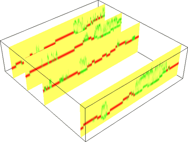
Figure: Proportional count of points per 3D cell. When 50% of all points in a vertical column fall into a given 3D cell, the value is 0.5. Here, the green color was assigned to 0.5, red to 1 and yellow to 0. The figure shows vertical slices and green color indicates high vegetation while red color indicates bare ground.

NOTES

This module is new and partially experimental. Please don't rely on its interface and be critical towards its outputs. Please report issues on the mailing list or in the bug tracker.
No reprojection is performed, you need to reproject ahead or use GRASS Location which has the right coordinate system which fits with the data.
Some temporary maps are created but not cleaned up. Use of --overwrite might be necessary even when not desired.
Expects points to have intensity and causing random (undefined) result for related outputs (sum, mean, proportional_sum) when the intensity is not present but the outputs were requested.

EXAMPLES

Basic import of the data

Set the region according to a 2D raster and adding 3D minimum (bottom), maximum (top) and vertical (top-bottom) resolution.

g.region rast=secref b=80 t=160 tbres=5 -p3

Now, r3.in.lidar will create the 3D raster of the size given by the computation region:

r3.in.lidar input=points.las n=points_n sum=points_sum \
    mean=points_mean proportional_n=points_n_prop \
    proportional_sum=points_sum_prop

Point density vertical structure reduced to the terrain

Create ground raster:

r.in.lidar input=points.las output=ground method=mean class_filter=2

Set vertical extent of computational region to (relative) coordinates above ground:

g.region rast=secref b=0 t=47 -p3

Compute point density:

r3.in.lidar input=points.las n=points_n sum=points_sum \
    mean=points_mean proportional_n=points_n_prop \
    proportional_sum=points_sum_prop \
    base_raster=ground

Complete workflow for vertical structure analysis

Compute the point density of points in 2D while setting the output extent to be based on the data (-e) and the resolution set to a relatively high number (here 10 map units, i.e. meters for metric projections).

r.in.lidar input=points.las output=points_n method=n -e resolution=10

This step can be repeated with using different resolutions (and the --overwrite flag) to determine the resolution for the further analysis.

The class_filter option should be also provided if only part of the points is analyzed, for example class_filter=3,4,5 would be used for low, medium, and high vegetation if the LAS file follows the usedstandard ASPRS class numbers.

The resolution should be suitable for computing digital elevation model which will be computed in the next steps. Once you decided on the resolution, you can use the 2D raster to set the computational region extent and resolution:

g.region raster=points_n -p3

class_filter=2 is used to limit

r.in.lidar input=points.las output=ground_mean method=mean class_filter=2

The following steps are not necessary if the point density is high enough to fill the raster continuously.

Convert the raster to vector point resulting in a decimated point cloud:

v.to.rast input=ground_mean type=point output=ground_decimated use=z

Interpolate the ground surface from the decimated ground points:

v.surf.rst input=ground_decimated elevation=ground

Now we need to determine upper vertical limit for the 3D raster (the top value from g.region -p3). This can be potentially done with lower resolution. The -d flag ensures that the ground raster will be used in its actual resolution regardless of the resolution of the output.

r.in.lidar input=points.las method=max output=veg_max class_filter=3,4,5 base_raster=ground -d

With that, we can finally set up the 3D extent and resolution:

g.region rast=secref b=0 t=40 res=1 res3=1 -p3

Note that the 2D and 3D resolutions are separate so that user can perform the 2D calculations on a finer resolution than the 3D calculations. The vertical resolution can be and often is set to a different value as well. Here we use the same value for all resolutions for simplicity.

Finally, we perform the 3D binning where we count number of points per cell (voxel):

r3.in.lidar input=points.las n=n class_filter=3,4,5 base_raster=ground -d

REFERENCES

V. Petras, A. Petrasova, J. Jeziorska, H. Mitasova (2016): Processing UAV and lidar point clouds in GRASS GIS. XXIII ISPRS Congress 2016 [ISPRS Archives, ResearchGate]
ASPRS LAS format
LAS library
LAS library C API documentation

AUTHOR

Vaclav Petras, NCSU GeoForAll Lab

Last changed: $Date$