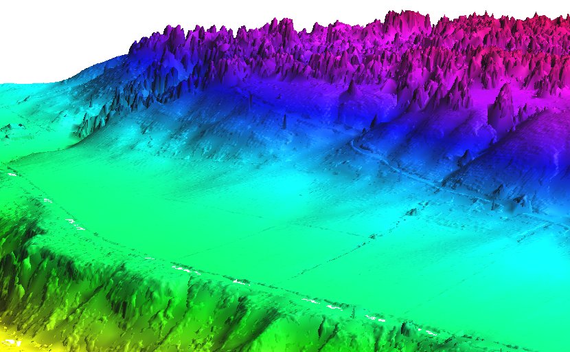
Mean value DEM in perspective view, imported from LAS file
Since the creation of raster maps depends on the computational region settings (extent and resolution), as default the current region extents and resolution are used for the import. When using the -e flag along with the resolution=value parameter, the region extents will be based on new dataset. It is therefore recommended to first use the -s flag to get the extents of the LiDAR point cloud to be imported, then adjust the current region extent and resolution accordingly, and only then proceed with the actual import. Another option is to automatically set the region extents based on the LAS dataset itself along with the desired raster resolution. See below for details.
r.in.lidar is designed for processing massive point cloud datasets, for example raw LiDAR or sidescan sonar swath data. It has been tested with large datasets (see below for memory management notes).
Available statistics for populating the output raster map are:
| n | number of points in cell |
| min | minimum value of points in cell |
| max | maximum value of points in cell |
| range | range of points in cell |
| sum | sum of points in cell |
| mean | average value of points in cell |
| stddev | standard deviation of points in cell |
| variance | variance of points in cell |
| coeff_var | coefficient of variance of points in cell |
| median | median value of points in cell |
| percentile | pth percentile of points in cell |
| skewness | skewness of points in cell |
| trimmean | trimmed mean of points in cell |
The default map type=FCELL is intended as compromise between preserving data precision and limiting system resource consumption.
For the output raster map, a suitable resolution can be found by dividing the number of input points by the area covered (this requires an iterative approach as outlined here):
# print LAS metadata (Number of Points)
r.in.lidar -p input=points.las
#   Number of Point Records: 1287775

# scan for LAS points cloud extent
r.in.lidar -sg input=points.las output=dummy -o
# n=2193507.740000 s=2190053.450000 e=6070237.920000 w=6066629.860000 b=-3.600000 t=906.000000

# set computation region to this extent
g.region n=2193507.740000 s=2190053.450000 e=6070237.920000 w=6066629.860000 -p

# print resulting extent
g.region -p
#  rows:       3454
#  cols:       3608

# points_per_cell = n_points / (rows * cols)
# Here: 1287775 / (3454 * 3608) = 0.1033359 LiDAR points/raster cell
# As this is too low, we need to select a lower raster resolution

g.region res=5 -ap
#  rows:       692
#  cols:       723
#  Now: 1287775 / (692 * 723) = 2.573923 LiDAR points/raster cell

# import as mean
r.in.lidar input=points.las output=lidar_dem_mean method=mean -o

# import as max
r.in.lidar input=points.las output=lidar_dem_max method=max -o

# import as p'th percentile of the values
r.in.lidar input=points.las output=lidar_dem_percentile_95 \
           method=percentile pth=95 -o
Further hints: how to calculate number of LiDAR points/square meter:
g.region -e
  # Metric location:
  # points_per_sq_m = n_points / (ns_extent * ew_extent)

  # Lat/Lon location:
  # points_per_sq_m = n_points / (ns_extent * ew_extent*cos(lat) * (1852*60)^2)
Blank lines and comment lines starting with the hash symbol (#) will be skipped.
The zrange parameter may be used for filtering the input data by vertical extent. Example uses might include preparing multiple raster sections to be combined into a 3D raster array with r.to.rast3, or for filtering outliers on relatively flat terrain.
In varied terrain the user may find that min maps make for a good noise filter as most LIDAR noise is from premature hits. The min map may also be useful to find the underlying topography in a forested or urban environment if the cells are oversampled.
The user can use a combination of r.in.lidar output maps to create custom filters. e.g. use r.mapcalc to create a mean-(2*stddev) map. [In this example the user may want to include a lower bound filter in r.mapcalc to remove highly variable points (small n) or run r.neighbors to smooth the stddev map before further use.]
# set the computational region automatically, resol. for binning is 5m
r.in.lidar -e -o input=points.las resolution=5 output=lidar_dem_mean
g.region rast=lidar_dem_mean -p
r.univar lidar_dem_mean
Serpent Mound dataset: This example is analogous to the example used in the GRASS wiki page for importing LAS as raster DEM.
The sample LAS data are in the file "Serpent Mound Model LAS Data.las", available at appliedimagery.com
# print LAS file info
r.in.lidar -p input="Serpent Mound Model LAS Data.las"

# using v.in.lidar to create a new location
# create location with projection information of the LAS data
v.in.lidar -i input="Serpent Mound Model LAS Data.las" location=Serpent_Mound

# quit and restart GRASS in the newly created location "Serpent_Mound"

# scan the extents of the LAS data
r.in.lidar -sg input="Serpent Mound Model LAS Data.las"

# set the region to the extents of the LAS data, align to resolution
g.region n=4323641.57 s=4320942.61 w=289020.90 e=290106.02 res=1 -ap

# import as raster DEM
r.in.lidar input="Serpent Mound Model LAS Data.las" \
           output=Serpent_Mound_Model_LAS_Data method=mean
Last changed: $Date$