This module is sensitive to mask settings. All cells which are outside the mask are ignored and handled as no flow boundaries.
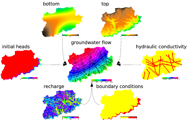
r.gwflow calculates the piezometric head and optionally
the water budget and the filter velocity field,
based on the hydraulic conductivity and the piezometric head.
The vector components can be visualized with paraview if they are exported
with r.out.vtk.
The groundwater flow will always be calculated transient.
For stady state computation set the timestep
to a large number (billions of seconds) or set the
storativity/ effective porosity raster map to zero.
The water budget is calculated for each non inactive cell. The
sum of the budget for each non inactive cell must be near zero.
This is an indicator of the quality of the numerical result.
(dh/dt)*S = div (K grad h) + q
In detail for 2 dimensions:
(dh/dt)*S = Kxx * (d^2h/dx^2) + Kyy * (d^2h/dy^2) + q
Confined and unconfined groundwater flow is supported. Be aware that the storativity input parameter is handled differently in case of unconfined flow. Instead of the storativity, the effective porosity is expected.
To compute unconfined groundwater flow, a simple Picard based linearization scheme is used to solve the resulting non-linear equation system.
Two different boundary conditions are implemented, the Dirichlet and Neumann conditions. By default the calculation area is surrounded by homogeneous Neumann boundary conditions. The calculation and boundary status of single cells must be set with a status map, the following states are supportet:
# set the region accordingly
g.region res=25 res3=25 t=100 b=0 n=1000 s=0 w=0 e=1000 -p3

#now create the input raster maps for confined and unconfined aquifers
r.mapcalc expression="phead = if(row() == 1 , 50, 40)"
r.mapcalc expression="status = if(row() == 1 , 2, 1)"
r.mapcalc expression="well = if(row() == 20 && col() == 20 , -0.01, 0)"
r.mapcalc expression="hydcond = 0.00025"
r.mapcalc expression="recharge = 0"
r.mapcalc expression="top_conf = 20.0"
r.mapcalc expression="top_unconf = 70.0"
r.mapcalc expression="bottom = 0.0"
r.mapcalc expression="null = 0.0"
r.mapcalc expression="poros = 0.15"
r.mapcalc expression="s = 0.0001"

# The maps of the river
r.mapcalc expression="river_bed = if(col() == 35 , 48, null())"
r.mapcalc expression="river_head = if(col() == 35 , 49, null())"
r.mapcalc expression="river_leak = if(col() == 35 , 0.0001, null())"

# The maps of the drainage
r.mapcalc expression="drain_bed = if(col() == 5 , 48, null())"
r.mapcalc expression="drain_leak = if(col() == 5 , 0.01, null())"

#confined groundwater flow with cg solver and sparse matrix, river and drain
#do not work with this confined aquifer (top == 20m)
r.gwflow solver=cg top=top_conf bottom=bottom phead=phead status=status \
  hc_x=hydcond hc_y=hydcond q=well s=s recharge=recharge output=gwresult_conf \
  dt=8640000 type=confined vx=gwresult_conf_velocity_x vy=gwresult_conf_velocity_y budget=budget_conf

#unconfined groundwater flow with cg solver and sparse matrix, river and drain are enabled
# We use the effective porosity as storativity parameter
r.gwflow solver=cg top=top_unconf bottom=bottom phead=phead \
  status=status hc_x=hydcond hc_y=hydcond q=well s=poros recharge=recharge \
  river_bed=river_bed river_head=river_head river_leak=river_leak \
  drain_bed=drain_bed drain_leak=drain_leak \
  output=gwresult_unconf dt=8640000 type=unconfined vx=gwresult_unconf_velocity_x \
  budget=budget_unconf vy=gwresult_unconf_velocity_y

# The data can be visulaized with paraview when exported with r.out.vtk
r.out.vtk -p in=gwresult_conf,status vector=gwresult_conf_velocity_x,gwresult_conf_velocity_y,null \
  out=/tmp/gwdata_conf2d.vtk
r.out.vtk -p elevation=gwresult_unconf in=gwresult_unconf,status vector=gwresult_unconf_velocity_x,gwresult_unconf_velocity_y,null \
  out=/tmp/gwdata_unconf2d.vtk

#now load the data into paraview
paraview --data=/tmp/gwdata_conf2d.vtk &
paraview --data=/tmp/gwdata_unconf2d.vtk &
This work is based on the Diploma Thesis of Sören Gebbert available here at Technical University Berlin in Germany.
Last changed: $Date$